This post corresponds with a presentation given at eBay on 08 March 2016. Slides are available here
What are Self-Organizing Maps?
Self-Organizing Maps have been around for a while (I prefer to call them ‘Kohonen Maps’ but I guess ‘SOM’ rolls off the tongue better). There is no shortage of articles and papers available online that cover SOMs in depth, so I’ll keep this short.
A self-organizing map is an artificial neural network that does not follow the patterns typically associated with a neural network. Yes, SOMs require training, and yes trained SOMs automatically map input vectors. However, the structure of a trained SOM has more in common with a trained k-means model than say, an RNN. Rather than training an SOM using an error-correction model, we use vector quantization and a neighborhood function to build our SOM.
To oversimplify SOMs, they are a means to reduce high-dimensional data in a 2-D or 3-D space so that observations similar to each other are represented closer together. By plotting for each attribute, it’s possible to create an intuitive visualization that depicts observations and where they are in the system with respect to a given variable.
Below is a video of depicting an SOM being trained using education data collected by the WorldBank. It depicts the mapped ‘locations’ of each country and the overlay of the SOM’s grid weights for each variable with which the countries were compared.
It is important to note that this depiction reveals the variations among observations (in this case, countries) according to variable, where the end result is a 2-D plot mapping distances between countries within the high-dimensional space. While Finland and Afghanistan may appear “close” to each other in regards to education, they are only “close” to each other given the data and observations selected. Since this SOM was trained on data that did not include important measures of educational quality, such as student performance, it is not expected to be an adequate depiction of “true” closeness between countries. The purpose of depicting the iterative progress of training an SOM, however, is fulfilled quite nicely.
There is currently no native SOM implementation available in TensorFlow. PyMVPA, py-kohonen, sevamoo/SOMPY and JustGlowing/minisom work well enough, but this post is not about using current implementations.Sachin Joglekar’s implementation, published back in November 2015, is a great start, but a lot more could be done with it.
Let’s Make a Self-Organizing Map
First we need data…
Download the data from the WorldBank
Cleaning and normalizing the WorldBank data is done in R. It is important to normalize the data as it simplifies the process of depicting individual attributes as a heightmap (see above video).
#Load the necessary libraries.
libraries  <- c('data.table', 'plyr', 'dplyr', 'tidyr')
lapply(libraries, require, character.only = TRUE)

#Let's get our data and rename columns accordingly
df <- fread("WDI/WDI_Data.csv", na.strings = "..", header = TRUE)
names(df)[1:4] <- c("CountryName", "CountryCode", "IndicatorName", "IndicatorCode")

#Select columns that we actually care about
df <- subset(df, select=c("CountryName", "CountryCode", "IndicatorName", "IndicatorCode",
                        '2005', '2006', '2007', '2008', '2009', '2010','2011',
                        '2012', '2013', '2014', '2015'))

#Distinguish actual countries from aggregates. The raw data includes aggregates, so
#I have stored a small csv with only "aggregate" countries.

aggregates <- fread("WDI/country_aggregates.csv", na.strings = "..", header = TRUE)[1:68]
aggregates <- unique(aggregates$`Country Code`)
#Separate aggregates and countries, for later use.
df_c <- filter(df, !(df$CountryCode %in% aggregates))
df_agg <- filter(df, (df$CountryCode %in% aggregates))

clean_data <- function(dataframe, quality_frac){
  df.tmp <- dataframe

  #For now, we only include percentages and "current dollar" indexes.
  df.tmp<- filter(df.tmp, grepl(pattern = "ZS|GROW|ZG|CD", x = dataframe$IndicatorCode))

  #We count the number of NA values; this metric will later allow us to assess which
  #metrics are less frequently/consistently collected
  df.tmp$count_na <- rowSums(is.na(subset(df.tmp,
                            select = c('2005', '2006', '2007', '2008',
                                      '2009', '2010','2011', '2012',
                                      '2013', '2014', '2015'))))

  #we take the average of all observations from 2005 to 2015.
  df.tmp$Mean <- apply(subset(df.tmp,
                    select = c('2005', '2006', '2007', '2008', '2009', '2010','2011',
                               '2012', '2013', '2014', '2015')),
                               1, FUN = mean, na.rm = TRUE)

  #we can calculate the median too, although as of this writing, we will be using the mean
  df.tmp$Median <- apply(subset(df.tmp,
                    select = c('2005', '2006', '2007', '2008',
                              '2009', '2010','2011', '2012',
                              '2013', '2014', '2015')),
                              1, FUN = median, na.rm = TRUE)

  #"We will calculate "indicator quality" as a function of how many countries have
  #no observations for the given indicator.
  df.tmp %>% group_by(IndicatorName, IndicatorCode) %>% tally(count_na == 11) -> indicator_quality.tmp
  n_countries.tmp <- (df_c %>% group_by(CountryName) %>% tally() %>% dim())[1]
  qual_indicators.tmp <- filter(indicator_quality.tmp, n <= (n_countries.tmp*(quality_frac)))
  df.tmp <- filter(df.tmp, IndicatorCode %in% qual_indicators.tmp$IndicatorCode)
  df.tmp %>% group_by(CountryName, CountryCode) %>% tally(is.na(Median)) -> country_qual.tmp

  #We will also get rid of countries with a missing value count greater than 2.5 times the average.
  #This is done for the sake of maximizing the # of available variables to compare countries by,
  #and to save time that would otherwise be spent imputing our data
  qual_countries.tmp <- filter(country_qual.tmp, n <= 2.5* mean(country_qual.tmp$n))
  print(median(country_qual.tmp$n))
  df.tmp <- filter(df.tmp, CountryName %in% qual_countries.tmp$CountryName)
  df.tmp <- subset(df.tmp,
    select = c("CountryName", "CountryCode", "IndicatorName", "Mean"))
  df.tmp$Mean <- as.numeric(df.tmp$Mean)

  #Spread data to leave country names and country codes in the first two columns.
  #all other columns contain calculated means for each emtric
  df.tmp <- spread(df.tmp, key = IndicatorName, value = Mean)

  df_out_names.tmp <- select(df.tmp, c(CountryName, CountryCode))
  df_out.tmp <- select(df.tmp, -c(CountryName, CountryCode))

  df_out.tmp <- apply(df_out.tmp, MARGIN = 2,
    FUN = function(X) round((X - min(X, na.rm = TRUE))/diff(range(X, na.rm = TRUE)),
    digits = 5))

  df_OUT.tmp<- cbind(df_out_names.tmp$CountryName,df_out_names.tmp$CountryCode, df_out.tmp)
  return(df_OUT.tmp)
}

df_c_ <- clean_data(df_c, 0.5)
df_c_ <- as.data.frame(df_c_)
for(i in c(3:length(df_c_))){
  df_c_[,i] <- as.numeric(as.character(df_c_[,i]))
}

#The rest of this is just an iterative way of sampling from the cleaned dataset.
sample_df<- sample_frac(df_c_,size = 0.45)

for(i in c(1:27)){
  learn_rate_A = 1.07^i
  learn_rate_B = 1.05^i
  sample_df <- sample_df[,colSums(is.na(sample_df)) < nrow(sample_df)/learn_rate_A]
  sample_df <- sample_df[rowSums(is.na(sample_df)) < ncol(sample_df)/learn_rate_B,]
}
sample_df <- sample_df[,colSums(is.na(sample_df)) < nrow(sample_df)/20]
sample_df <- sample_df[rowSums(is.na(sample_df)) < ncol(sample_df)/20,]

for(i in c(1:35)){
  learn_rate_A = 1.05^i
  learn_rate_B = 1.07^i
  sample_df <- sample_df[,colSums(is.na(sample_df)) < nrow(sample_df)/learn_rate_A]
  sample_df <- sample_df[rowSums(is.na(sample_df)) < ncol(sample_df)/learn_rate_B,]
}
sample_df <- sample_df[rowSums(is.na(sample_df)) < 1,]
sample_df <- sample_df[,colSums(is.na(sample_df)) < 1]

sample_to_bind <- sample_df[3:length(sample_df)]
output <- cbind(sample_df[,1], sample_df[,2], sample_to_bind)
names(output)[1:2] <- c("CountryName", "CountryCode")
write.table(output, file = "CountryData.csv", sep = ";",row.names = FALSE, col.names = TRUE)
Building Our SOM Class
This assumes you already have TensorFlow installed. Instructions can be found here.
Let’s import the libraries we’ll use. In addition to TensorFlow, we’ll need numpy and pyplot.
import tensorflow as tf
import numpy as np
from matplotlib import pyplot as plt
class SOM(object):
"""
A 2-D Kohonen Map (more commonly known as a self-organizing map, or SOM)
Neighbourhood function: Gaussian
Learning Rate: decreases linearly.
"""
def __init__(self, m,n, dim, n_iterations=100, alpha=0.05, sigma=None):
"""
m X n = dimensions of the SOM.
n_iterations = number of training iterations
dim = dimensionality of the training inputs.
alpha = float value for initial learning rate.
sigma = radius of influence of the best matching unit (BMU).
default value is half of max(m, n)
"""
#Assign required variables
self._m = m
self._n = n
self._centroid_grid = [] #initialize centroid grid to observe training
self._map_vectors = [] #initialize map vectors, which store topography
self._n_iterations = int(n_iterations)
alpha = float(alpha)
if sigma is None: #setting default neighborhood radius
sigma = max(m, n) / 2.2
else:
sigma = float(sigma)
#Init our TensorFlow graph
self._graph = tf.Graph()
# as_default allows us to assign operations and tensors in "self"
with self._graph.as_default():
#Assign random weights for nodes in grid and
#store as a matrix of size [m*n, dim]
self._weight_vects = tf.Variable(tf.random_normal(
[m*n, dim]))
#Create matrix of size [m*n, 2] for SOM grid
self._location_vects = tf.constant(np.array(
list(self._node_locations(m, n))))
#Training vector TF placeholder
self._vect_input = tf.placeholder("float", [dim])
#Iteration TF placeholder
self._iter_input = tf.placeholder("float")
#Compute the Best Matching Unit given a vector using Euclidean distance
#between every node's weight vector and the input
#Returns the index of the node which gives the least value
bmu_index = tf.argmin(tf.sqrt(tf.reduce_sum(
tf.pow(tf.sub(self._weight_vects, tf.pack(
[self._vect_input for i in range(m*n)])), 2), 1)),0)
#Gets location of the BMU based on the BMU's index
slice_input = tf.pad(tf.reshape(bmu_index, [1]),
np.array([[0, 1]]))
bmu_loc = tf.reshape(tf.slice(self._location_vects, slice_input,
tf.constant(np.array([1, 2]))),[2])
#Compute alpha and sigma based on iteration number
learning_rate_op = tf.sub(1.0, tf.div(self._iter_input, self._n_iterations))
_alpha_op = tf.mul(alpha, learning_rate_op)
_sigma_op = tf.mul(sigma, learning_rate_op)
#Construct the op that will generate a vector with learning
#rates for all nodes, based on iteration number and location.
bmu_distance_squares = tf.reduce_sum(tf.pow(tf.sub(
self._location_vects, tf.pack(
[bmu_loc for i in range(m*n)])), 2), 1)
neighbourhood_func = tf.exp(tf.neg(tf.div(tf.cast(
bmu_distance_squares, "float32"), tf.pow(_sigma_op, 2))))
learning_rate_op = tf.mul(_alpha_op, neighbourhood_func)
#Finally, the op that will use learning_rate_op to update
#the weight vectors of all nodes based on a particular input
learning_rate_multiplier = tf.pack([tf.tile(tf.slice(
learning_rate_op, np.array([i]), np.array([1])), [dim])
for i in range(m*n)])
weight_delta = tf.mul(
learning_rate_multiplier,
tf.sub(tf.pack([self._vect_input for i in range(m*n)]),
self._weight_vects))
new_weights_op = tf.add(self._weight_vects,
weight_delta)
self._training_op = tf.assign(self._weight_vects,
new_weights_op)
##INITIALIZE SESSION
self._sess = tf.Session()
##INITIALIZE VARIABLES
init_op = tf.initialize_all_variables()
self._sess.run(init_op)
def _node_locations(self, m, n):
"""
Yields the 2-D locations of the individual nodes in the SOM.
"""
#Nested iterations over both dimensions
#to generate all 2-D locations in the map
for i in range(m):
for j in range(n):
yield np.array([i, j])
def train(self, input_vects):
"""
Trains the SOM.
'input_vects' is an iterable of 1-D NumPy arrays.
Uses random weight vectors as starting conditions for training.
"""
#Count training iterations. Process an iteration
for iter_no in range(self._n_iterations):
#Take all input vectors and train using one at a time.
for input_vect in input_vects:
self._sess.run(self._training_op, feed_dict={self._vect_input: input_vect,self._iter_input: iter_no})
#Save each calculated centroid location to a grid.
centroid_grid = [[] for i in range(self._m)]
self._weights = list(self._sess.run(self._weight_vects))
self._locations = list(self._sess.run(self._location_vects))
for i, loc in enumerate(self._locations):
centroid_grid[loc[0]].append(self._weights[i])
self._centroid_grid.append(centroid_grid) #store the centroid grid to list of
#previous grids for reference
self._to_map = []
for vector in input_vects:
min_index = min([i for i in range(len(self._weights))],
key=lambda x: np.linalg.norm(vector-self._weights[x]))
self._to_map.append(self._locations[min_index])
self._map_vectors.append(self._to_map)
def get_centroids(self):
"""
Returns a list of 'm' lists, with each inner list containing
the 'n' corresponding centroid locations as 1-D NumPy arrays.
"""
return self._centroid_grid
def map_vects(self, input_vects):
"""
Maps each input vector to the relevant node in the SOM grid.
'input_vects' should be an iterable of 1-D NumPy arrays with
dimensionality as provided during initialization of this SOM.
Returns a list of 1-D NumPy arrays containing (row, column)
info for each input vector(in the same order), corresponding
to mapped node.
"""
return self._map_vectors
[self._vect_input for i in range(m*n)])), 2), 1)),
0)
#This will extract the location of the BMU based on the BMU's
#index
slice_input = tf.pad(tf.reshape(bmu_index, [1]),
np.array([[0, 1]]))
bmu_loc = tf.reshape(tf.slice(self._location_vects, slice_input,
tf.constant(np.array([1, 2]))),
[2])
#To compute the alpha and sigma values based on iteration
#number
learning_rate_op = tf.sub(1.0, tf.div(self._iter_input,
self._n_iterations))
_alpha_op = tf.mul(alpha, learning_rate_op)
_sigma_op = tf.mul(sigma, learning_rate_op)
#Construct the op that will generate a vector with learning
#rates for all neurons, based on iteration number and location
#wrt BMU.
bmu_distance_squares = tf.reduce_sum(tf.pow(tf.sub(
self._location_vects, tf.pack(
[bmu_loc for i in range(m*n)])), 2), 1)
neighbourhood_func = tf.exp(tf.neg(tf.div(tf.cast(
bmu_distance_squares, "float32"), tf.pow(_sigma_op, 2))))
learning_rate_op = tf.mul(_alpha_op, neighbourhood_func)
#Finally, the op that will use learning_rate_op to update
#the weightage vectors of all neurons based on a particular
#input
learning_rate_multiplier = tf.pack([tf.tile(tf.slice(
learning_rate_op, np.array([i]), np.array([1])), [dim])
for i in range(m*n)])
weightage_delta = tf.mul(
learning_rate_multiplier,
tf.sub(tf.pack([self._vect_input for i in range(m*n)]),
self._weightage_vects))
new_weightages_op = tf.add(self._weightage_vects,
weightage_delta)
self._training_op = tf.assign(self._weightage_vects,
new_weightages_op)
##INITIALIZE SESSION
self._sess = tf.Session()
##INITIALIZE VARIABLES
init_op = tf.initialize_all_variables()
self._sess.run(init_op)
def _neuron_locations(self, m, n):
"""
Yields one by one the 2-D locations of the individual neurons
in the SOM.
"""
#Nested iterations over both dimensions
#to generate all 2-D locations in the map
for i in range(m):
for j in range(n):
yield np.array([i, j])
def train(self, input_vects):
"""
Trains the SOM.
'input_vects' should be an iterable of 1-D NumPy arrays with
dimensionality as provided during initialization of this SOM.
Current weightage vectors for all neurons(initially random) are
taken as starting conditions for training.
"""
#Training iterations
for iter_no in range(self._n_iterations):
#Train with each vector one by one
for input_vect in input_vects:
self._sess.run(self._training_op, feed_dict={self._vect_input: input_vect,self._iter_input: iter_no})
print("Iteration %d complete"%iter_no)
#Store a centroid grid for easy retrieval later on
centroid_grid = [[] for i in range(self._m)]
self._weightages = list(self._sess.run(self._weightage_vects))
self._locations = list(self._sess.run(self._location_vects))
for i, loc in enumerate(self._locations):
centroid_grid[loc[0]].append(self._weightages[i])
self._centroid_grid = centroid_grid
self._trained = True
def get_centroids(self):
"""
Returns a list of 'm' lists, with each inner list containing
the 'n' corresponding centroid locations as 1-D NumPy arrays.
"""
return self._centroid_grid
def map_vects(self, input_vects):
"""
Maps each input vector to the relevant neuron in the SOM grid.
'input_vects' should be an iterable of 1-D NumPy arrays with
dimensionality as provided during initialization of this SOM.
Returns a list of 1-D NumPy arrays containing (row, column)
info for each input vector(in the same order)
"""
if not self._trained:
raise ValueError("SOM not trained yet")
to_return = []
for vect in input_vects:
min_index = min([i for i in range(len(self._weightages))],
key=lambda x: np.linalg.norm(vect-
self._weightages[x]))
to_return.append(self._locations[min_index])
return to_returnTypically the data we will use will look like the data below:
country_names =["Afghanistan","Australia","Belarus","Brazil","Bulgaria","Denmark","Finland","India","Italy","Japan",
     "Norway","Russian Federation","Uganda","United States"]

countries = np.array([
        [0.273,0.701,0.908,0.549,0.787,0.63,0.203,0.228],
        [0.058,0.92,0.914,0.871,0.958,0.897,0.042,0.048],
        [0.744,0.268,0.466,0.117,0.409,0.156,0.689,0.679],
        [0.257,0.773,0.903,0.435,0.866,0.558,0.182,0.202],
        [0.112,0.969,0.916,0.423,0.974,0.724,0.064,0.07],
        [0.072,0.919,0.881,0.855,0.92,0.901,0.063,0.067],
        [0.237,0.725,0.65,0.809,0.73,0.787,0.28,0.258],
        [0.248,0.772,0.943,0.424,0.888,0.561,0.163,0.186],
        [0.191,0.818,0.916,0.564,0.912,0.664,0.132,0.147],
        [0.036,0.97,0.936,0.802,0.98,0.896,0.015,0.022],
        [0.42,0.551,0.738,0.481,0.643,0.501,0.353,0.384],
        [0.482,0.52,0.56,0.478,0.563,0.495,0.465,0.458],
        [0.416,0.566,0.931,0.294,0.741,0.384,0.293,0.334]
                       ])


country_metrics = ["GINI index (World Bank estimate)","Income share held by second 20%",
                    "Income share held by fourth 20%","Income share held by lowest 10%",
                    "Income share held by third 20%","Income share held by lowest 20%","Income share held by highest 10%",
                    "Income share held by highest 20%"]
Rather than copy-pasting the data, we will use pandas to load the .csv created in R
countries = pd.read_csv('CountryData.csv', sep=';', header = 0)
country_names = countries['CountryName'].values
country_codes = countries['CountryCode'].values
country_values = countries.ix[:,2:].values
country_metrics = countries.ix[:,2:].columns.values
Next we declare the number of iterations and dimensions used. We will leave alpha and sigma alone for now.
n_iter = 100
xdim = 30
ydim = 20
map_dim = len(country_values[1])
Finally, we train our SOM and retrieve mapping data for each observation.
som = SOM(xdim, ydim, map_dim, n_iter)
som.train(country_values)
#Get output grid
image_grid_long = som.get_centroids()

#Map colours to their closest neurons
mapped_long = som.map_vects(country_values)
Finally we iterate through our SOM and weight maps, creating plots with pyplot.
h = 0
colors = []
while h < n_iter:
    image_grid_append = []
    for metr in range(0,len(country_metrics)):
        gray_array = []
        for i in range(0,xdim):
            gray_list = []
            for j in range(0,ydim):
                gray_list.append(image_grid_long[h][i][j][metr])
            gray_array.append(gray_list)
        image_grid_append.append(gray_array)
    colors.append(image_grid_append)
    h += 1


metr = 0
while metr < map_dim:
    for g in range(0,n_iter):
        plt.figure(figsize=(9,6))
        plt.title("%s, Iter %s"%(str(country_metrics[metr]), str(g)))
        for i, m in enumerate(mapped_long[g]):
            plt.plot(m[0], m[1], 'ro')
            plt.text(m[0], m[1] -0.75, country_codes[i], ha='center', va='center', bbox=dict(facecolor='white', alpha=0.7, lw=0))
        plt.imshow(colors[g][metr], extent=[0,xdim,0,ydim], aspect='auto', alpha = 0.5)

        if metr in range(0,10):
            _metr = str(0) + str(metr)
        else:
            _metr = metr

        if g in range(0,10):
            filename = (str(_metr) + str(0) + str(g))
        else:
            filename = (str(_metr) + str(g))
        plt.savefig(filename)
    metr += 1
#End of plotting_
Using ffmpeg we convert the output into a single mp4.
ffmpeg -framerate 25 -pattern_type glob -i '*.png' -c:v libx264 -pix_fmt yuv420p out.mp4The Results
It is worth drawing attention to the fact that the nature of this implementation treats all metrics equally. So while many might see the U.S. as more similar to Australia than say, Russia, our SOM disagrees. Why? Well, it’s trained on using a random sample of World Development Indicators as collected by the WorldBank. The indicators range from population size to per capita GDP to incidence of tuberculosis (per 100,000 people).
We can also adjust our learning rate to see how it make affect the composition of our SOM. Due to the randomized nature of how each SOM is generated, the start and end locations for each country will most certainly differ from training set to training set, however the calculated distances relative to other countries will more or less stay the same, with variations dependent on the number of iterations, the neighborhood radius (sigma), and our learning rate alpha.
100 Iterations, alpha = 0.05
Setting alpha to 0.05, the map fails to properly converge.
100 Iterations, alpha = 0.3
An alpha of 0.3 seems to achieve acceptable results.
400 Iterations, alpha = 0.6
Further increasing alpha and the number of iterations yields greater separation between countries.
800 Iterations, alpha = 0.8
At this point, I really should be rewriting my code to make it more efficient. Training our SOM for 800 iterations takes approximately 36 minutes, after which we confirm a suspicion that 0.8 is an inappropriate value for alpha. Training simply takes too long and better results are not necessarily achieved.
A Comparison of Learning Rates
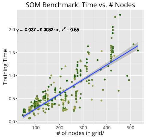
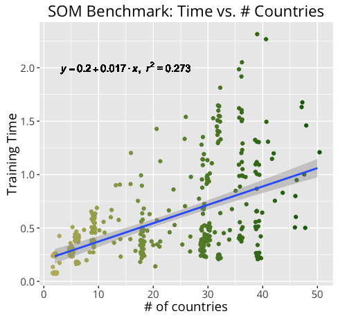
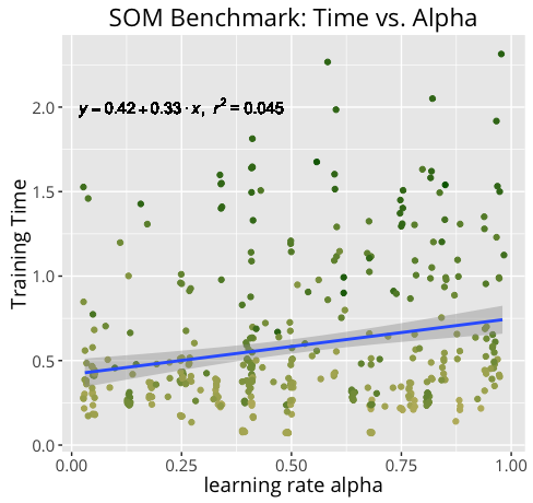
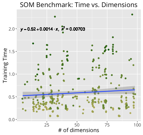
Performance
Not surprisingly, training an m X n SOM of n_dim dimensions takes much longer for a 20 X 30 100-dim map than it does for a 10 x 15 50-dim map. By measuring our training times under a variety of conditions, we can get a better idea of how certain components may contribute more heavily to training time.
Below are the results of the benchmark.
Further Development
There are a number of ways this implementation could be further improved. A good start would be adding some argparse functionality as to better guide the output. Additionally, it would make more sense to rename local variables to be data-neutral, as SOM are not just useful for comparing countries. Since SOMs are also inherently computationally expensive, particularly as the observations increase, incorporating multithreading might generate faster results. In its current state, it runs in polynomial time and is far too expensive computationally to compare large datasets.